Water Flow Calculation Methods for Central Air Conditioning Systems

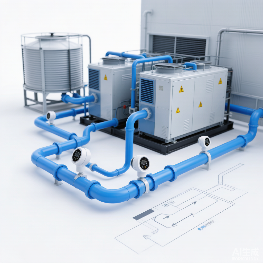
Figure: Central air conditioning water system schematic showing cooling tower, chiller, pumps, and AHU piping layout

Introduction to HVAC Water Systems

Central air conditioning water systems form the circulatory backbone of modern HVAC infrastructure, responsible for transporting thermal energy between chillers, cooling towers, and air handling units (AHUs). The design and calculation of water flow rates directly influence system efficiency, equipment sizing, operational stability, and long-term reliability. Incorrect flow calculations can lead to inadequate cooling capacity, excessive energy consumption, pipe erosion, or even catastrophic equipment failure. This article presents a systematic approach to water flow calculation methods, covering cooling water circuits, chilled water loops, makeup water requirements, and the interaction between variable flow strategies and chiller performance.

Modern HVAC water systems typically consist of three interrelated circuits: the cooling water loop (between chiller condenser and cooling tower), the chilled water loop (between chiller evaporator and terminal units), and the makeup water supply. Each circuit has distinct hydraulic and thermal design requirements that must be carefully balanced to achieve optimal system performance. Understanding the fundamental heat transfer equation Q = m × Cp × ΔT is essential, where Q represents the thermal load, m is the mass flow rate, Cp is the specific heat capacity of water, and ΔT is the temperature differential across the heat exchanger.

Cooling Water Flow Calculation

The cooling water flow rate is a critical design parameter that determines the size of cooling towers, condenser water pumps, and associated piping. The standard formula for calculating cooling water flow rate is:

L (m³/h) = [Q (kW) / (4.5~5) ℃ × 1.163] × (1.15~1.2)

Explanation of Variables and Coefficients

• Q (kW): Cooling capacity. This is the total heat rejection load of the chiller condenser, which equals the chiller’s cooling capacity plus the compressor input power. For a typical chiller with a COP of 5.0, the heat rejection is approximately 120% of the cooling capacity.
• 4.5~5℃: Temperature difference across the condenser. The narrower the ΔT, the higher the required flow rate. A ΔT of 5℃ is standard for most comfort cooling applications, while 4.5℃ may be used for process cooling requiring tighter temperature control. Selecting an appropriate ΔT balances pumping energy against heat exchanger sizing.
• 1.163: Conversion constant. This factor converts kilowatts to thermal flow units: 1 kW = 860 kcal/h, and the specific heat of water is 1 kcal/(kg·℃). The constant 1.163 = 860 / (1000 × 1), converting kW to m³/h per ℃. This ensures dimensional consistency in the calculation.
• (1.15~1.2): Safety factor. This multiplier accounts for heat gain in piping, fouling factors in heat exchangers, part-load operation variability, and provides a design margin. The factor range of 1.15 to 1.2 is recommended by ASHRAE guidelines for commercial HVAC applications. Critical process cooling may warrant factors up to 1.3.

Design Examples

For a 500 kW (142 RT) chiller with a 5℃ condenser ΔT: L = [500 / (5 × 1.163)] × 1.2 = 103.2 m³/h. This flow rate would require a condenser water pipe diameter of approximately DN150 (6 inches) based on a recommended velocity of 1.5 to 2.5 m/s. The corresponding cooling tower would need to be sized for 580 kW of heat rejection capacity at design ambient conditions.

Chilled Water Flow Calculation

Chilled water flow calculation follows similar thermodynamic principles but must account for simultaneous load diversity and system configuration. The primary formula for chilled water flow is:

Chilled Water Flow (m³/h) = Cooling Capacity (kW) × 0.86 / ΔT (℃)

Where 0.86 is the simplified conversion factor (860 kcal/h per kW divided by 1000 kg/m³). The standard design ΔT for chilled water is 5℃ (supply at 7℃, return at 12℃), though modern high-efficiency systems increasingly use a ΔT of 7-8℃ to reduce pumping energy at the expense of slightly larger coil surfaces.

Impact of Simultaneous Use Rate

The simultaneous use rate (also called diversity factor) is the ratio of the peak coincident load to the sum of individual peak loads of all terminal units. In multi-zone buildings, not all spaces require maximum cooling simultaneously due to varying solar exposure, occupancy patterns, and internal heat gains. Typical diversity factors range from 0.7 to 0.9 for office buildings and 0.6 to 0.8 for hotels.

• Design Flow Adjustment: The total chilled water flow should be calculated based on the DIVERSIFIED peak load, not the sum of individual terminal unit peaks. Over-sizing the chilled water flow leads to oversized pumps, increased capital cost, and poor part-load efficiency.
• Primary-Secondary Systems: In primary-secondary configurations, the primary (chiller-side) flow is sized for the chiller’s design ΔT, while the secondary (building-side) flow is sized for the actual required coil ΔT. A common bypass decoupler prevents the two flows from interfering with each other.
• Variable Primary Flow: Modern VPF systems eliminate the secondary pump by using variable-speed primary pumps. The minimum flow must be maintained above the chiller manufacturer’s specification (typically 40-60% of design flow) to prevent laminar flow and freezing risk in the evaporator.

Cooling Water Makeup Rate

Cooling towers lose water through three mechanisms: evaporation, drift (windage), and blowdown (purge). The total makeup water requirement must compensate for all three losses to maintain system water quality and prevent scale formation. The standard makeup rate is typically calculated as:

• Evaporation Loss: Approximately 0.85% of the circulating water flow for every 5.5℃ (10℉) of cooling range. For a typical 5℃ range, the evaporation rate is approximately 0.77% of circulation rate.
• Drift Loss: Modern drift eliminators limit drift loss to 0.001-0.005% of circulation rate. Older towers without drift eliminators may lose up to 0.1-0.2%.
• Blowdown Rate: Calculated based on the desired cycles of concentration (COC). Blowdown = Evaporation / (COC – 1). For a COC of 5, blowdown equals 25% of evaporation loss. Higher COC values reduce water consumption but increase scaling risk.
• Total Makeup Rate: Typically 1.0-1.6% of the circulating water volume. For a 1000 m³/h cooling water system, the daily makeup requirement ranges from 240 to 384 m³/day. This represents a significant operating cost and should be factored into the life-cycle economic analysis.

Variable Water Flow Impact on Chiller Performance

The transition from constant flow to variable flow systems represents one of the most significant advances in HVAC water system design over the past two decades. While variable flow offers substantial energy savings, it introduces operational risks that must be managed through proper design and control strategies.

Traditional Constant Flow Design Considerations

Conventional constant flow systems maintain a fixed water flow rate regardless of the actual cooling load. While simple and robust, this approach wastes pumping energy during part-load conditions, which constitute 90% or more of operating hours in most buildings. A constant flow 100 kW pump operating at full speed year-round can consume over 870,000 kWh annually, equivalent to approximately 600 tonnes of CO₂ emissions from grid electricity.

Modern Variable Flow Control Technology

Variable frequency drives (VFDs) modulate pump speed to match water flow with the actual thermal load. Since pump power varies with the cube of speed (affinity laws), reducing flow to 80% of design results in only 51% of the design power consumption. Combined with advanced control strategies, VFD-based systems can achieve 30-50% pumping energy savings compared to constant flow designs.

• Differential Pressure Control: The most common control strategy maintains a constant differential pressure at the most remote (critical) coil. As terminal unit valves close, system resistance increases, and the pump slows down to maintain the setpoint. This ensures adequate flow to all coils while minimizing pump speed.
• Temperature-Based Reset: The differential pressure setpoint can be reset based on system demand indicators such as the position of the most-open control valve or the difference between supply and return chilled water temperature. This further reduces pumping energy during low-load periods.
• Demand-Based Sequencing: Multiple parallel pumps can be staged on and off based on measured flow rate or system pressure, ensuring each operating pump runs near its best efficiency point (BEP). Proper sequencing prevents the efficiency penalty of running a single large pump at very low speed.

Laminar Flow Risk

When flow rates drop too low, the transition from turbulent to laminar (or transitional) flow in the chiller evaporator tubes dramatically reduces the heat transfer coefficient. The Nusselt number drops significantly below the critical Reynolds number of approximately 2300, and the overall heat transfer coefficient can decrease by 40-60%. This degrades chiller efficiency (increases kW/RT) and may cause the chiller to cycle excessively or trip on low evaporator temperature safety limits.

Freezing Risk

Insufficient water velocity in the evaporator, combined with low refrigerant temperature, creates a risk of localized freezing on the water side of the heat exchanger tubes. A single frozen tube can rupture and cause refrigerant loss and water ingress into the refrigeration circuit, resulting in catastrophic compressor damage. Minimum flow rates specified by chiller manufacturers must be strictly maintained, typically 40-60% of design flow for standard shell-and-tube evaporators.

Corrosion Risk

Low flow velocities allow suspended solids to settle in horizontal tube passes, creating under-deposit corrosion cells. Stagnant or very slow-moving water also promotes microbiological growth, including sulfate-reducing bacteria that cause microbiologically influenced corrosion (MIC). A minimum velocity of 0.9 m/s (3 ft/s) is recommended to maintain self-cleaning conditions in closed-loop chilled water piping.

Practical Design Considerations

Pipe Sizing Guidelines

Proper pipe sizing balances capital cost (larger pipes are more expensive) against operating cost (smaller pipes increase pumping energy). Recommended velocity ranges per ASHRAE and CIBSE guidelines are:

Pipe Service	Recommended Velocity (m/s)	Maximum Velocity (m/s)	Pressure Drop (Pa/m)
Chilled water mains	1.5 – 2.4	3.0	200 – 400
Condenser water	1.8 – 2.7	3.6	200 – 400
Pump suction	0.6 – 1.2	1.5	100 – 200
Branch lines	1.2 – 2.1	2.4	100 – 300
Riser pipes	1.5 – 3.0	3.6	150 – 400

Pump Selection Criteria

Centrifugal pumps remain the industry standard for HVAC water circulation. Key selection considerations include:

• Best Efficiency Point (BEP): The pump should be selected so the design operating point falls between 80% and 110% of BEP flow. Operating far from BEP increases radial thrust, vibration, and seal wear. The preferred operating region recommended by the Hydraulic Institute is 70-120% of BEP flow.
• Net Positive Suction Head (NPSH): The available NPSH must exceed the pump’s required NPSH by a margin of at least 1 meter to prevent cavitation. Systems with open cooling towers require particular attention to suction conditions, especially for pumps located above the sump water level.
• Standby Capacity: Critical facilities should provide N+1 pump redundancy. For variable flow systems, it is often more energy-efficient to use multiple smaller pumps with VFDs than a single large pump with a standby unit.

Flow Balancing

Hydronic system balancing ensures that each terminal unit receives its design flow rate under all operating conditions. The three primary balancing methods are:

• Manual Balancing Valves: Circuit setters or calibrated balancing valves with pressure/temperature ports. The most economical option but requires rebalancing after system modifications. Best suited for constant flow systems with stable load profiles.
• Automatic Flow Limiting Valves: Pressure-independent control valves (PICVs) maintain constant flow regardless of system pressure fluctuations. They combine the functions of a control valve and balancing valve, simplifying commissioning and ensuring stable control loop performance. PICVs are ideal for variable flow systems.
• Commissioning and Verification: Post-installation flow measurement using ultrasonic flow meters or calibrated balancing valves should verify that all circuits are within ±10% of design flow. System over flow increases pumping energy, while underflow compromises cooling performance. A complete test and balance report is an essential handover document.

In conclusion, accurate water flow calculation is the foundation of efficient HVAC system design. By applying the proper thermodynamic principles, safety factors, and design practices outlined in this article, engineers can deliver systems that provide reliable comfort cooling while minimizing energy consumption and lifecycle costs. As variable flow technology continues to mature, the industry moves toward ever more efficient hydronic designs that intelligently match system output to actual building loads.

Source: Compressor Maintenance Forum